In the previous chapter we discussed using encodings to represent input/output objects as strings, and we talked about formalizing computational tasks as decision problems (equivalently languages), function problems, or search problems. In this chapter, we will formalize the notion of “algorithm” or “computing device”, and what it means for one to solve a computational task. Our basic algorithmic model will be Turing Machines.
Let us recap some of the ideas from the previous chapter. Suppose you care about finding paths in graphs using a computing device. The associated search problem would be: Given (the encoding of) a graph \(G\) and vertices \(s\), \(t\), find a path from \(s\) to \(t\) in \(G\) if one exists. The associated decision problem is just to answer yes/no, does such a path exist? The equivalent language is \[\textbf{Path} = \{\langle G, s, t \rangle : \text{ there is a path from $s$ to $t$ in $G$}\}.\]
Our next step will to be define a notion of an algorithm/computing machine using the concept of Turing Machines. You may have seen these before in the context of computability theory. A Turing Machine \(M\) will take in an input string, do some computation (hopefully without entering an infinite loop), and then either “accept” or “reject”. We’ll say that \(M\) solves or decides language \(L\) if \(M(x)\) accepts for all \(x \in L\) and \(M(x)\) rejects for all \(x \not \in L\). (Turing Machines will also be capable of outputting strings, and therefore solving function and search problems, too.)
Returning to the language \(\textbf{Path}\):
The computability question about this language is: Does there exist an algorithm \(M\) solving \(\textbf{Path}\)? As you probably know, there is!
The complexity question about this language is: Does there exist an algorithm \(M\) solving \(\textbf{Path}\) while always using at most \(T\) resources?
As we discussed, there are many kinds of resources to consider: running time, memory usage, etc. This suggests the importance of formalizing algorithms in such a way that it is very clear how to quantify their resource-usage.
The \(\textbf{Path}\) problem is pretty simple, and the efficiency of algorithms for it is well understood. Here is another problem whose complexity is more difficult to analyze: \[\begin{aligned} \textbf{Circuit-Sat} = \{\langle C \rangle :\ & \text{$C$ is an AND/OR/NOT circuit such that there exists a $\mathtt{0}/\mathtt{1}$ setting } \\ &\text{for its input wires such that its (single) output wire is $\mathtt{1}$.} \}\end{aligned}\] There does indeed exist a Turing Machine algorithm \(M\) that decides this language. However, is there one that gives the correct answer on every input string \(x\) in at most \(\operatorname{poly}(|x|)\) steps? This question is equivalent to the famous \(\mathsf{P}\overset{?}{=} \mathsf{NP}\) question, as we will see.
“Turing Machines are the worst formalization of Algorithms except for all those other formalizations that have been tried.”
To begin Complexity Theory, we need to pick a programming language to be the official one we use to define “algorithms”. Here are some programming languages one might consider (and one could consider many, many others):
| Python | Turing Machine |
| Java | (untyped) Lambda Calculus |
| C | Post Machine |
| C++ | Wang Machine |
| Haskell | \(P''\) (the theoretical precursor to BF) |
| Ruby | Piet |
| Julia | LOLCODE |
| \(\cdots\) | \(\cdots\) |
Notice that we have referred to Turing Machine as a “programming language” here, whereas you might think of them as…“machines”. Or at least as some kind of non-programming-language computing paradigm. But the right way to think of a Turing Machine is that it is a piece of code in a particular esoteric programming language.
In the left column above we see some “standard” programming languages. The Pro of choosing one of these is that they are enjoyable to program in. The Con of choosing one of these is that they are very hard to completely and rigorously define and reason about. In the right column above we see some “esoteric” programming languages. (The first five, Turing Machines through \(P''\), are programming languages that have historically been used for reasoning about the nature of computation. That last two are joke languages, often used in, e.g., Code Golf.) The Pros and Cons of using these languages are just the opposite: they are annoying to program in, but we can fully reason about the mathematically.
For the purposes of mathematical modeling, it’s natural to allow input strings of any length, and also to allow computations that can use any amount of time and memory. So if you were to imagine using, say, C as the official programming language for Complexity Theory, you should imagine that it has access to a potentially unlimited amount of memory; that is, you can malloc() as much as you want.
We also do not consider “interactive computation” in beginning Complexity Theory (though we will get to it a bit at the end of the course). So you shouldn’t think of algorithms/code with input statements, interacting with a user. Instead, think of an algorithm as a function, with some inputs and one returned value.
Although there are many potential choices for a programming language to define computation, you may know that, from the point of view of computability, we can choose Turing Machines “without loss of generality”. This is thanks to the Church–Turing Thesis:
The Church–Turing Thesis is that any real-world algorithm can be simulated by (i.e., compiled to) Turing Machines.
On the other hand, essentially all programming languages ever used are Turing-complete, meaning that one can write a Turing Machine-interpreter in them. So from a computability point of view, any programming language could be used to formalize computation. But in addition to their mathematical simplicity, there are three main reasons we prefer Turing Machines.
The first reason is historical. Turing Machines were the first formalization of algorithms broadly agreed to be universal. Turing himself gave a compelling physical argument for this, by illustrating how Turing Machines can simulate human computers. Turing Machines are also widely in textbooks on Computability and Complexity Theory, so it is good to get to know them well just so you can read other papers and books.
The second reason is that it is extremely easy to exactly define how many times steps and memory cells a Turing Machine uses. This makes them particularly suitable for Complexity Theory analysis. By comparison, in any high-level language like Python or C, it would be difficult to adjudicate how many “times steps” a line of code should count for.
The third reason concerns one of the most important basic results in Complexity Theory, the Time Hierarchy Theorem (see Chapter (The Time Hierarchy Theorem)). The fundamental idea behind its proof involves taking one’s programming language — call it \(T\) — and writing a \(T\)-interpreter in the language \(T\). When we choose \(T\) to be Turing Machines, it means we have to reason about a Turing Machine whose job is to simulate Turing Machines (usually called a Universal Turing Machine). If we were to choose, say, the BF programming language instead, we’d have to reason about BF code that simulates BF code; if we were to choose Python, we’d basically have to think about how to write the
exec()command in Python. There is an obvious tradeoff here — the more powerful your programming language is, the more enjoyable it is to write code in it…but also the more complicated the task of producing a complete interpreter for it. It turns out that it’s much better to go the route of making the programming language as simple as possible. Even the presence of built-in loops (as in the BF language, for example) makes things annoying, since it means you have to implement a stack data structure to simulate nested loops.
Returning to the Church–Turing Thesis, it says that for the purposes of deciding what is computable at all, it is “without loss of generality” to study Turing Machines. But what about for Complexity Theory, for the purposes of deciding what is computable efficiently? You probably know that programming with Turing Machines is elaborate, painful, and repetitive. Could it be that there are computational problems solvable “efficiently” in some high-level language like C, but not solvable “efficiently” by Turing Machines? The answer turns out to be “No, at least if you are somewhat relaxed about the notion of efficient.” For example, with some effort you can define a limited “C-like pseudocode” programming language, and also a precise running time model for it. Then:
An algorithm running in \(T\) time steps in “C-like pseudocode” can be compiled to a Turing Machine algorithm running in \(O(T^4)\) time steps.
“Polynomial time” is the same concept for “C-like pseudocode” and Turing Machines; any problem solvable in polynomial time using C-like pseudocode can also be solved in polynomial time using Turing Machines.
We will talk about these kinds of simulations soon in Chapter (Programming in TM). In basic Complexity Theory we are not very worried about “polynomial factors”, and thus relatively early in the course we will stop describing algorithms with Turing Machines (which is annoying) and instead just describe them using C-like pseudocode. (Of course, in practical Algorithms theory, one does care about polynomial factors, and the \(4\)th-power slowdown in Corollary (C-like pseudocode simulation) is not great. We will also discuss this later.) As you might imagine, one can write a reasonably efficient interpreter for any high-level programming language in C-like pseudocode. This leads us to:
The Extended Church–Turing Thesis is that any real-world algorithm running in \(T\) “steps” can be simulated by a Turing Machine running in \(\operatorname{poly}(T)\) steps. Hence the classification of which computational problems are “solvable in polynomial time” does not depend on the programming language used to formalize algorithms.
The Extended Church–Turing Thesis is actually strongly challenged by the possibility of quantum computing!
Our official model of computation in this course is the one-tape Turing Machine with “\(2\)-way-infinite tape”.
As a warning, the popular textbook by Sipser uses a “\(1\)-way-infinite tape” instead.
We will first remind you of the “machine” picture of Turing Machines, before moving on to emphasize a programming language “code” model. The picture looks like this:
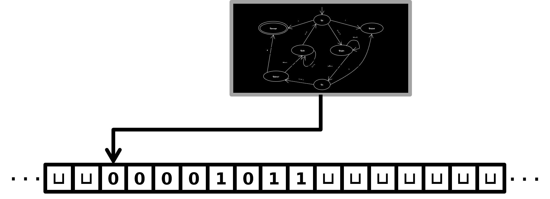
Information is stored on a “tape” in an infinite sequence of memory cells. Each cell can hold one symbol from an alphabet. A real-world computer with \(16\)GB of RAM can be thought of as a sequence of cells numbered from \(0\) up to \(2^{34}-1\), each capable of holding a “byte” (symbol in the range \(0\dots 255\)). By contrast, a Turing Machine tape is always assumed to be infinite, and the symbols can come from any fixed alphabet. As mentioned, we find it convenient to have the tape be ‘\(2\)-way-infinite’’, meaning the cells are numbered \(\dots, -3, -2, -1, 0, 1, 2, 3, \dots\), as opposed to \(0, 1, 2, 3, \dots\) on a “\(1\)-way-infinite” tape. There is also always a blank symbol, often denoted \(\sqcup\), and “empty” cells are assumed to be initialized to \(\sqcup\). In particular, while a Turing Machine is running, almost all cells will contain \(\sqcup\); only a finite number of tape cells will store a non-blank symbol.
The “control” of a Turing Machine — the black box in the picture, that has states, transitions, etc. — should be thought of as the source code for the Turing Machine. Unlike in most high-level computational models where the code has “random-access” to the memory (it’s right there in the name RAM!), the Turing Machine control has a simple pointer called the “read/write head”, which always points to one memory cell. In each time step, the Turing Machine control can take an action based on its current “state” as well as the symbol being read by its read/write head. (These states are like “line numbers” in textual programming languages.) The action involves writing a new symbol into the current cell, and then moving the read/write head left or right. (The main reason we have decided on the \(2\)-way-infinite tape model is so we don’t have to handle the edge case of “what happens if the head is moved left when it is already at the left edge of the tape”.)
It’s good to think of the “source code” (control) of a Turing Machine as a table that looks something like this:
| state | read symbol | write symbol | move dir. | new state |
|---|---|---|---|---|
| \(q_0\) | \(\mathtt{0}\) | \(\mathtt{1}\) | R | \(q_1\) |
| \(q_0\) | \(\mathtt{1}\) | \(\mathtt{0}\) | R | \(q_{\text{walkRight}}\) |
| \(q_0\) | \(\sqcup\) | \(\sqcup\) | L | \(q_{\text{acc}}\) |
| \(q_1\) | \(\mathtt{0}\) | \(\mathtt{x}\) | R | \(q_2\) |
| \(q_1\) | \(\mathtt{1}\) | \(\sqcup\) | L | \(q_0\) |
| \(q_1\) | \(\sqcup\) | \(\sqcup\) | R | \(q_{\text{copy}}\) |
| \(\vdots\) | \(\vdots\) | \(\vdots\) | \(\vdots\) | \(\vdots\) |
Here \(q_0\), \(q_1\), \(q_{\text{walkRight}}\), etc. are “states” (like line numbers), and L and R stand for Left and Right. There should be a row in the table for every (state, read symbol) pair. The above table is just made up and does not come from any sensible Turing Machine. But the following is a good Turing Machine example:
Go to http://morphett.info/turing/turing.html to see and interact with an example of Turing Machine code deciding the language \[\textbf{Palindromes} = \{\epsilon, \mathtt{0}, \mathtt{1}, \mathtt{00}, \mathtt{11}, \mathtt{000}, \mathtt{010}, \dots \} \subset {\{\mathtt{0},\mathtt{1}\}}^*.\]
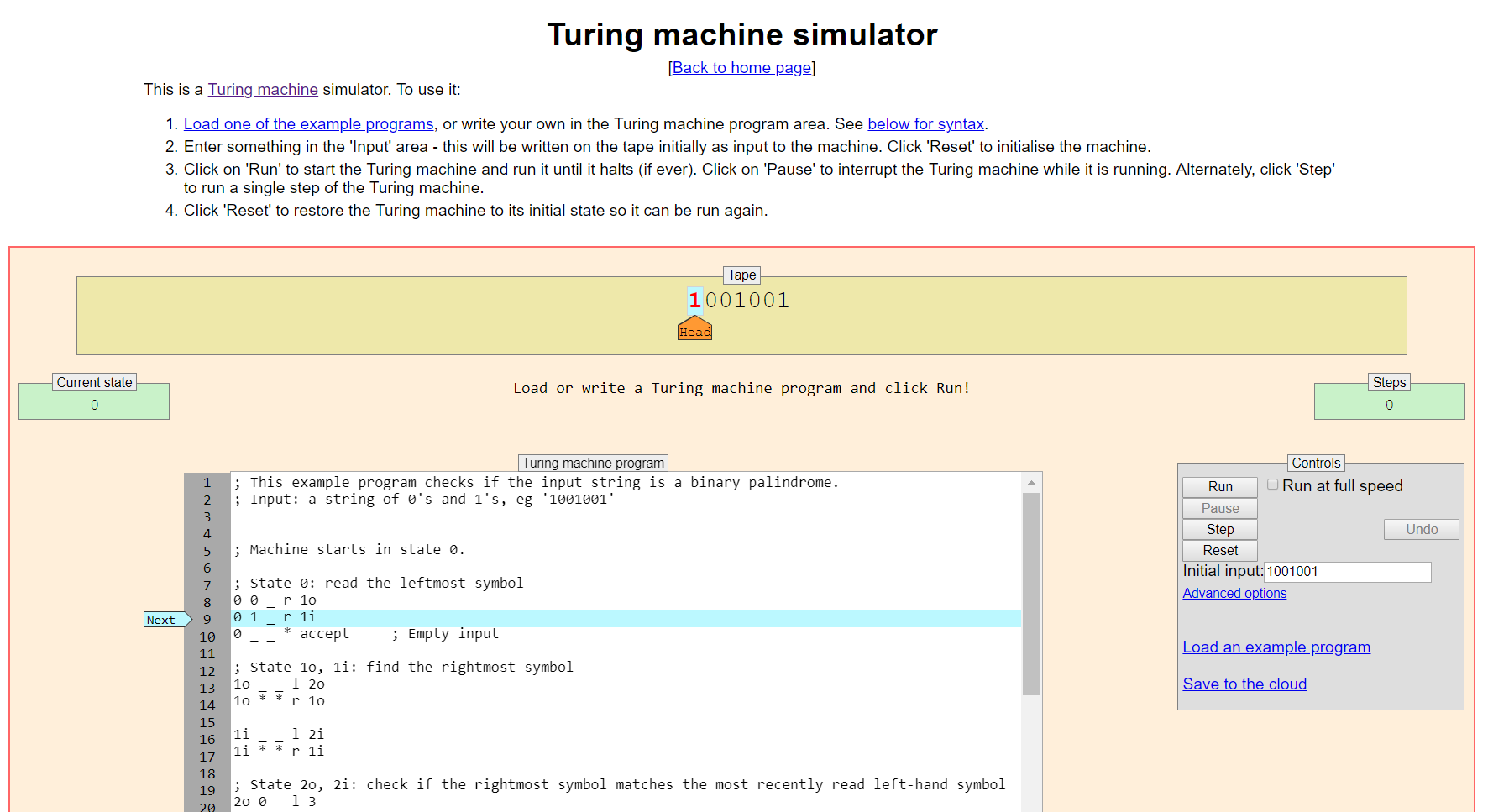
This is a wonderful online Turing Machine simulator produced by Anthony Morphett.
Turing Machine Visualization (turingmachine.io) by Andy Li is another online Turing Machine simulator; its graphics and editor are very beautiful, but Morphett’s is more functional.
Note that both of the aforementioned online Turing Machine simulators have a source code editing box, wherein you effectively enter the contents of a table, in text. Although we will give a formal mathematical definition of Turing Machines and their computation using “math objects”, it’s good to think them as pieces of code, expressible in text.
We can now give an “official” definition of what a Turing Machine is. This is like defining the “syntax” of a programming language. In honor of this viewpoint, we’ll start to call them “TM algorithms”.
A Turing Machine, or TM algorithm, consists of:
\(\Sigma\), an input alphabet that does not contain the blank symbol \(\sqcup\).
\(\Gamma\), a tape alphabet that contains all the symbols in \(\Sigma\), plus the blank symbol \(\sqcup\), plus it may contain additional symbols.
\(Q\), a finite set of states.
Three specially designated states in \(Q\): an initial state (often written \(q_0\)), an accept state (often written \(q_{\text{acc}}\)), and a reject state (often written \(q_{\text{rej}}\)). The accept and reject state must be different, but the initial state is allowed to be the same as one of them.
A transition function \(\delta : Q' \times \Gamma \to \Gamma \times \{\text{L}, \text{R}\} \times Q\), where \(Q' = Q \setminus \{q_{\text{acc}}, q_{\text{rej}}\}\). In other words, \(\delta\) is a mapping from (state,symbol) pairs to (symbol,direction,state) pairs; in other other words \(\delta\) specifies the “table” or “source code”. The business with \(Q'\) is because we assume the TM algorithm doesn’t take any action when it gets to a halting state.
Other textbooks and sources may use slightly different definitions than Definition (Turing Machine, or TM algorithm) above. As we’ll see in Chapter (Programming in TM), it’s no big deal.
Let’s return to the TM code solving \(\textbf{Palindromes}\) at Morphett.
Its input alphabet is \(\Sigma = {\{\mathtt{0},\mathtt{1}\}}\).
Its tape alphabet is \(\Gamma = \{\mathtt{0}, \mathtt{1}, \sqcup, \textup{\texttt{:}}, \textup{\texttt{)}}, \textup{\texttt{(}}\}\), which has\(6\) symbols in it. The last three symbols illustrate that it’s fine to have more symbols in your tape alphabet than \(\Sigma \cup \{\sqcup\}\) if you wish, although Morphett’s code just uses them for drawing smileys
:)By default, Morphett requires the initial state to be called “\(0\)”. (This is annoying because \(0\) is much more common as a tape symbol, and it’s not good to have states and tape symbols with the same name. Luckily, if you go to “Advanced options” in Morphett you can change this default.) Let’s rename this initial state to \(q_0\). With this renaming, the TM code’s state set is \[Q = \{q_0, 1o, 1i, 2o, 2i, 3, 4, \textit{accept}, \textit{accept2}, \textit{reject}, \textit{reject2}, \textit{halt-accept}, \textit{halt-reject}\}.\] These names are not too evocative; it would have been nicer if he’d given clearer names.
The initial state is \(q_0\), the accept state is \(\textit{halt-accept}\), and the reject state is \(\text{halt-reject}\).
The transition function \(\delta\) is specified on the website and won’t be repeated here. But, for example, the first two lines of the code specify that \[\delta(q_0, \mathtt{0}) = (\sqcup, \text{R}, \textit{1o}), \qquad \delta(q_0, \mathtt{1}) = (\sqcup, \text{R}, \textit{1i}).\]
Actually, Morphett’s Turing Machine syntax allows the head to stay put in a step (not move Left or Right), which our definition does not allow. As mentioned, though, this is not a big deal. Morphett also allows a bit more “syntactic sugar”, as you can see.
We mentioned earlier that our model of Turing Machines would have a \(2\)-way-infinite tape, rather than the \(1\)-way-infinite tape that some textbooks use. Here’s a question:
Where in Definition (Turing Machine, or TM algorithm) is it reflected that we are using a \(2\)-way-infinite tape?
It’s a trick question, the answer is “nowhere”. This is because we have only defined Turing Machines’ syntax, not their semantics.
Having defined the syntax of TM code (what TM code is), we now define the semantics (what it means; that is, how it computes).
To follow the computation of TM code, you need to keep track of \(3\) things:
the tape contents;
the position of the tape head;
the current state.
Collectively these \(3\) things are called the configuration of the Turing Machine, and we package them into a string. For this purpose, we need to think of the state set \(Q\) also as an “alphabet” consisting of symbols (and — extreme technicality alert — these symbols should be distinct from the symbols in the tape alphabet \(\Gamma\).
Precisely, at a given point in the TM code’s computation, the configuration is a string \(C \in (\Gamma \cup Q)\) formed by:
taking the tape contents;
inserting the symbol for the current state into the string, just to the left of where the head is pointing;
trimming all the leading and trailing blanks (of which there are infinitely many).
In the following TM execution snapshot —
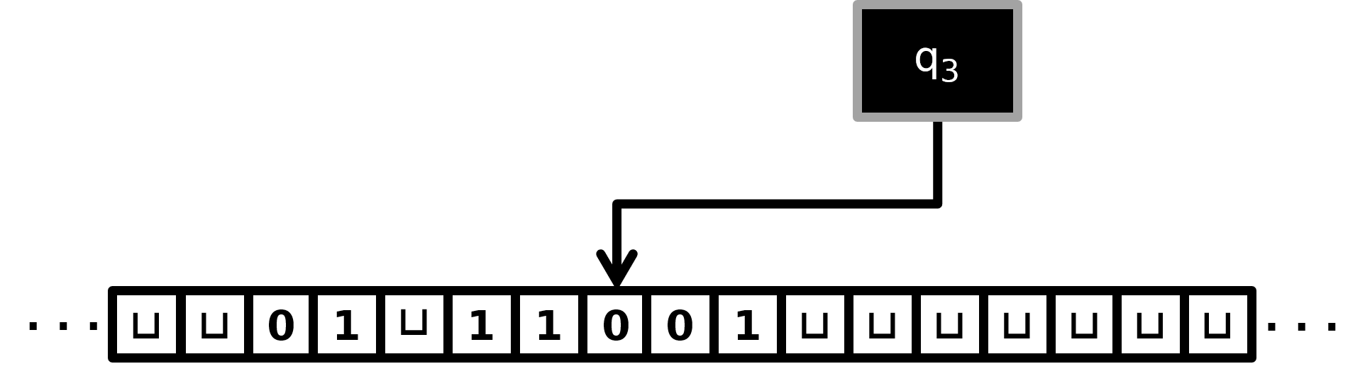
— the configuration is the string \(\mathtt{01}\sqcup\mathtt{11q_3}001\). (Here \(\mathtt{q_3}\) is one symbol.)
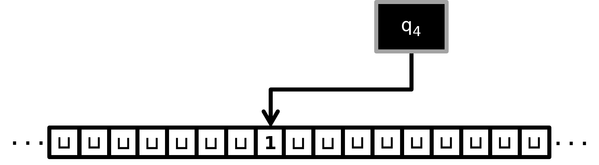
It is the \(2\)-symbol string \(\mathtt{q_41}\).
A string \(C \in (\Gamma \cup Q)^*\) is a valid configuration if and only if: (i) it has exactly one symbol from \(Q\); (ii) and, it has no leading or trailing blanks.
Now we can define the semantics of TM computation.
Given TM \(M\) and input string \(x\), the initial configuration is defined to be \(\mathtt{q_0}x\). (Here \(q_0\) is the symbol for \(M\)’s initial state, and the string \(x\) has been concatenated on the end.)
Configuration \(C\) is said to be a halting configuration if it contains either of the symbols \(\mathtt{q_{acc}}\) or \(\mathtt{q_{rej}}\)
Given a non-halting configuration \(C\) for TM \(M\), we define \(\text{NextConfig}_M(C)\) to be the configuration \(C'\) obtained (informally) by “doing one step of \(M\)”. Formally:
First one expresses \(C\) as \(u a q b v\), where \(q\) is the unique state symbol in \(C\), \(a\) and \(b\) are the symbols preceding and succeeding \(q\) (respectively), and \(u\) and \(v\) are the substrings preceding \(a\) and succeeding \(b\) (respectively). The strings \(u\) and \(v\) may equal the empty string \(\epsilon\), but if either \(a\) or \(b\) “does not exist”, it is treated as \(\sqcup\).
Then \(C'\) is set to be the following string, trimmed of any leading/trailing blanks it may have: \[u q' a d v \quad\text{if $\delta(q,b) = (d, \text{L}, q')$}, \qquad \text{or}\quad uadq'v \quad\text{if $\delta(q,b) = (d,\text{R},q')$}.\]
This definition is kind of technical and annoying to verify. However we’ve made it explicit just to fully convince you that TM computation can be formally defined entirely in terms of string manipulation.
The computation trace of TM \(M\) on input \(x \in \Sigma^*\) is \(C_0, C_1, C_2, \dots\), where \(C_0\) is the initial configuration, \(C_1 = \text{NextConfig}_M(C_0)\), \(C_2 = \text{NextConfig}_M(C_1)\), etc., either until a halting configuration \(C_t\) is reached, or else indefinitely.
If the computation trace of \(M\) on \(x\) terminates with some halting configuration \(C_t\), we say that \(M(x)\) halts. In this case, we furthermore say either that \(M(x)\) accepts or \(M(x)\) rejects, depending on whether \(C_t\) contains the symbol \(q_{\text{acc}}\) or \(q_{\text{rej}}\). On the other hand, if the computation trace of \(M\) on \(x\) is indefinite, we say that \(M(x)\) loops (or does not halt).
A great virtue of the TM model is that it’s easy to define “running time” exactly:
Say that \(M(x)\) halts, and the computation trace is \(C_0, C_1, \dots, C_t\). Then we say that \(M\) runs in time \(t\) on input \(x\).
We really hate when some TM code \(M\) has the possibility of looping, even on a single input. In this course, we basically ignore all such \(M\), deeming them to not even be real algorithms.
A TM \(M\) is a decider if \(M(x)\) halts for all inputs \(x \in \Sigma^*\).
We say that a TM \(M\) decides (or solves) a language \(L\) if:
\(M\) is a decider;
\(M(x)\) accepts for all \(x \in L\);
\(M(x)\) rejects for all \(x \not \in L\).
Define the language \[\textbf{Or} = \{ x \in \{0,1\}^* : x \text{ contains at least one } \mathtt{1}\}.\] We call this language “Or” because it contains the strings whose Boolean-OR is True. There is some simple TM code \(M\) that decides \(\textbf{Or}\). The high-level idea is that \(M\) simply scans the input from left-to-right: if it ever finds a \(\mathtt{1}\) it halts and accepts; if it ever encounters a blank symbol, it knows it has reached the end of the input without finding a \(\mathtt{1}\), so it halts and rejects. Indeed, \(M\) can use its initial state \(q_0\) to do all of this work, so besides this it only needs \(q_{\text{acc}}\) and \(q_{\text{rej}}\) states. The Morphett code is here:
    ; This program decides OR = {x : x contains a 1}, a subset of {0,1}*.
    ; The initial state is called q0.

    q0 _ _ L haltReject
    q0 1 1 R haltAccept
    q0 0 0 R q0
On input \(x = \mathtt{00010}\), the computation trace of \(M\) on \(x\) is: \[\begin{aligned} C_0 &= \mathtt{q_000010} \\ C_1 &= \mathtt{0q_00010} \\ C_2 &= \mathtt{00q_0010} \\ C_3 &= \mathtt{000q_010} \\ C_4 &= \mathtt{0001q_{acc}0} \end{aligned}\] We see that \(M(x)\) accepted, with a running time of \(4\).
On input \(x = \mathtt{00}\), the computation trace of \(M\) on \(x\) is: \[\begin{aligned} C_0 &= \mathtt{q_000} \\ C_1 &= \mathtt{0q_00} \\ C_2 &= \mathtt{00q_0} \\ C_3 &= \mathtt{0q_{rej}0} \end{aligned}\] We see that \(M(x)\) rejected, with a running time of \(3\).
Having seen these examples you should be able to convince yourself that indeed \(M\) decides the language Or.
This completes our description of the semantics of TM computation for languages/decision problems. A nice thing about TMs is that we can also think of them as producing output strings, so we can also use them to solve function/search problems too.
We say that TM \(M\) outputs a string \(y \in \Sigma^*\) on input \(x \in \Sigma^*\) if its final configuration is \(\mathtt{q_{acc}}y\). We say \(M\) computes \(f : \Sigma^* \to \Sigma^*\) if for all \(x \in \Sigma^*\), \(M(x)\) outputs the string \(f(x)\).
Note that here we required the TM to kind of “clean up” at the end of its computation by blanking out all the non-output, and moving the tape head to the left of the output. Usually insisting on this is not a big deal.
Go to http://morphett.info/turing/turing.html and carefully study the Parentheses checker example program. It illustrates some nice “TM programming tricks” that involve using extra symbols in the tape alphabet effectively.
Go to http://turingmachine.io/ and carefully study the Binary increment example program. It illustrates TM code that solves a function problem. Also, the “binary increment” operation is an important one for Complexity Theory, since generally one of the first things we often want TM code to be able to do is count up “\(n\)”, then number of symbols in the input.
Pros:
100% rigorously definable.
Running time (and memory usage) is 100% clear.
Turing motivated it by physical reality.
It’s simple.
It can simulate all known programming languages (this is the Church–Turing Thesis).
It’s not too hard to write a TM-code-simulator using TM code.
Cons:
It’s very painful to program in; it’s like an “esoteric programming language”.
The running times it gives are often polynomially worse than they “should be”.