In this chapter we show various “tricks” for writing code in the “TM programming language”. These help us show that the exact computational model we are using (Turing Machine with one \(2\)-way-infinite tape) does not matter that much, particularly if we don’t care about “polynomial factors” in time complexity.
As mentioned at the end of the last chapter, one virtue of Turing Machines is that there is a completely clear definition of the running time a TM \(M\) takes on an input \(x\) (Definition (Running time of a TM on an input).) We would now like to define the running time of the algorithm \(M\) itself.
A key idea in Complexity (and Algorithms) Theory is that we measure how the running time of algorithm \(M\) scales as a function of the input length, and in doing this we look at the worst-case input for each input length.
Let \(M\) be a decider algorithm. The running time (or time complexity) of \(M\) is the function, \(T_M : \mathbb{N}\to \mathbb{N}\), defined by \[T_M(n) = \max_{\substack{\text{inputs $x$} \\ |x| = n}} \{ \text{time $M$ takes on input $x$}\}.\]
Recall the TM \(M\) deciding the language Or from Example (TM deciding Or.). It is easy see that the number of steps \(M(x)\) takes to halt is \[\begin{cases} |x|+1 & \text{if $x$ does not contain a $\mathtt{1}$} \\ m & \text{if, otherwise, the first $\mathtt{1}$ in $x$ is in the $m$th position.} \end{cases}\] Thus \(M\)’s running time is the function \(T_M(n) = n+1\).
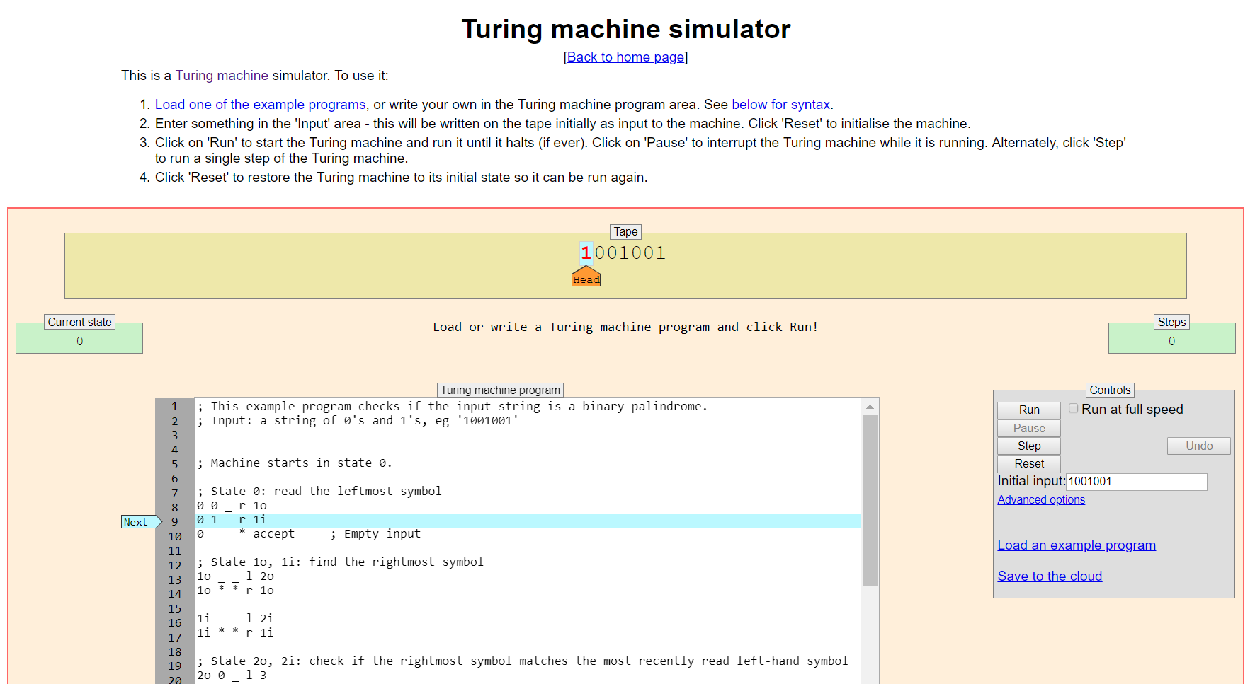
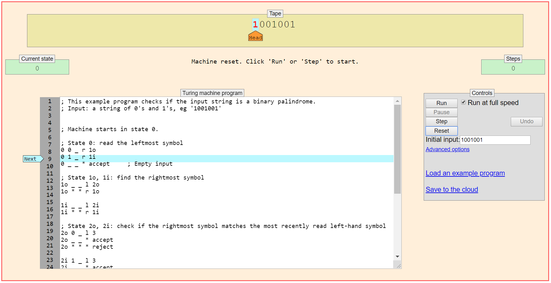
Ignoring the silliness of drawing smileys at the end, what is the exact running time function for the Morphett’s TM solving \(\textbf{Palindromes}\)?
Try to determine it empirically, first, by playing around in the simulator!
In the last chapter we described the “455 official” formal model of algorithms: \(1\)-tape TMs (with \(2\)-way-infinite tape). We also mentioned that there are several variants and alternatives that other pedagogic sources use (\(1\)-way-infinite tapes, multi-tape TMs, “C-like pseudocode”, etc.) By the Extended Church–Turing Thesis, we expect all these variants to be able to simulate each other with at most “polynomial slowdown”. In this chapter we will demonstrate some examples of this. In particular, we will explain some things about this simulations shown in this diagram:
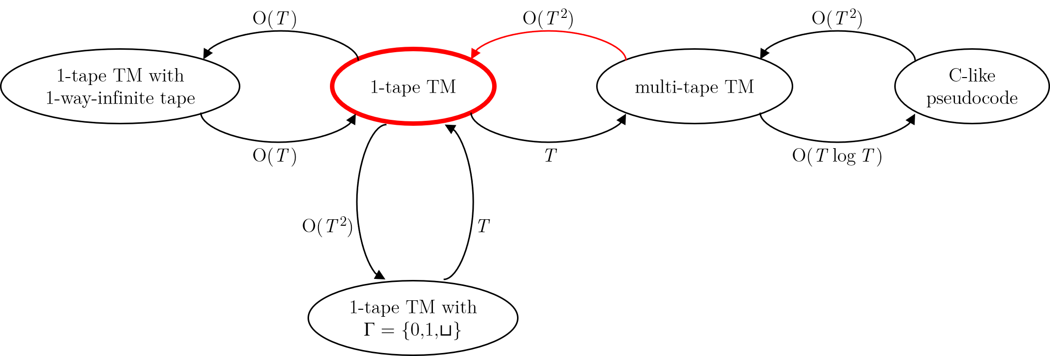
In the above diagram, the meaning of an arrow from model \(X\) to model \(Y\) and labeled \(O(T^2)\) is: An algorithm written in model \(X\) can be “simulated by” (or “compiled to”) an algorithm written in model \(Y\), with at most “quadratic slowdown”; i.e., if the running time function in model \(X\) was \(T(n)\), then the running time function in model \(Y\) is \(O(T(n)^2)\). Similarly for the labels \(O(T \log T)\) and \(T\). In fact, an arrow labeled \(T\) means there is no slowdown at all; a \(1\)-tape TM with \(\Gamma = \{\mathtt{0},\mathtt{1},\sqcup\}\) is a special case of a \(1\)-tape TM, so there is no need for any simulation/compilation, and similarly a \(1\)-tape TM is a special case of a multi-tape TM. We’ve circled “\(1\)-tape TM” in red because it’s our “official” model; we also highlighted in red the arrow about simulating multi-tape TMs on \(1\)-tape TMs because we’ll spend the most time talking about it.
Although what we’ll do in this chapter — messing around with the “esoteric programming language of TM” — can be tedious, there are some good reasons to do it at least once:
You’ll get practice “programming in TM”.
You’ll get explicit evidence for the Extended Church–Turing Thesis.
You’ll learn about two easier-to-program models: multi-tape Turing machines, and C-like pseudocode (known to professional algorithmicists as the Word RAM model). Since we don’t care about polynomial factors too much in this course, we may prefer to present algorithms in these models later in the course.
You’ll see an example of the adage from Chapter (Overview): “Most of Complexity Theory is…Algorithms.”
Consider an extended TM model where — when specifying what happens for each state/read-symbol combination — we may allow the tape head to “S”tay put, in addition to the usual “L”eft and “R”ight. (In fact, the Morphett interpreter allows this, with the symbol *.) A TM \(M\) in this model can be simulated by a TM \(M'\) in the usual model with at most factor-\(2\) slowdown; that is, with \(T_{M'}(n) \leq 2T_{M}(n)\).
We think of the “table of code” for \(M\), which may now have some “S” moves in it, in addition to the standard “L” and “R” moves. The idea is to convert each “S” move to an R followed by an L. We’ll need to also introduce some extra states for this. We give a “proof by example”, assuming the tape alphabet is \(\Gamma = \{\mathtt{0}, \mathtt{1}, \sqcup\}\). Suppose \(M\)’s code contains \[q_i, \mathtt{0} \mapsto \mathtt{1}, \textrm{S}, q_j\] meaning that when \(M\) is in state \(q_i\) and reading symbol \(\mathtt{0}\), it writes a \(\mathtt{1}\), keeps the tape head in the same place, and moves to state \(q_j\). To form the standard TM \(M'\), we replace this line of code with \[q_i, \mathtt{0} \mapsto \mathtt{1}, \textrm{R}, q_\textit{go-L-then-j}\] where go-L-then-j is a new state. We then add the following code: \[\begin{aligned} q_\textit{go-L-then-j}, \mathtt{0} &\mapsto \mathtt{0}, \textrm{L}, q_j \\ q_\textit{go-L-then-j}, \mathtt{1} &\mapsto \mathtt{1}, \textrm{L}, q_j \\ q_\textit{go-L-then-j}, \sqcup&\mapsto \sqcup, \textrm{L}, q_j \end{aligned}\] It is evident that \(M\) correctly simulates \(M'\), and that \(M(x)\) runs in at most twice as many steps as \(M'(x)\) for all inputs \(x\) (as any “S” moves by \(M'\) get replaced by two moves in \(M\)).
Consider an extended TM model which allows its head to move left twice or right twice in one step — call these moves LL and RR. Then again, a TM \(M\) in this model can be simulated by a TM \(M'\) in the usual model with at most factor-\(2\) slowdown; that is, with \(T_{M'}(n) \leq 2T_{M}(n)\).
This is similar to Proposition (Turing Machines where the head can Stay put). In fact, reusing the “\(q_\textit{go-L-then-j}\)” states/code from that proof, we just need to convert a double-move line in \(M\) like \[q_k, \mathtt{1} \mapsto \mathtt{0}, \text{LL}, q_j\] to \[q_k, \mathtt{1} \mapsto \mathtt{0}, \text{L}, q_\textit{go-L-then-j}\] Again, the correctness and running time bound should be clear.
A common trick in TM programming is “marking” a tape cell. This means to put a “dot” on a tape cell to help the TM find this particular cell later in the algorithm. Of course, there is no direct mechanism for a TM to “mark” a cell, but what you can do is introduce a “marked” version of each tape symbol. So for example, if your tape alphabet is \(\Gamma = \{\mathtt{0}, \mathtt{1}, \sqcup\}\), but you wanted to write code that used the “marking” technique, then the first thing you would do is change the tape alphabet to \[\Gamma = \{\mathtt{0}, \mathtt{1}, \sqcup, \mathtt{0}^{{}^{\!\!\bullet}}, \mathtt{1}^{{}^{\!\!\bullet}}, \sqcup^{{}^{\!\!\bullet}}\}.\] (We have 6 symbols here; e.g., we consider \(\mathtt{0}^{{}^{\!\!\bullet}}\) to be one symbol, despite the way it looks.)
A tape alphabet must always have exactly one “blank” symbol. In the above example with \(6\) symbols, the blank symbol is still \(\sqcup\). The “marked blank” \(\sqcup^{{}^{\!\!\bullet}}\) is treated as just another weird symbol.
A good example of this technique is if one is trying to simulate a TM with \(1\)-way-infinite tape by a (standard) TM with \(2\)-way-infinite tape. At first you might think there is nothing to do, but there is one catch. In the usual semantics of \(1\)-way-infinite tape TMs, if the TM tries to move Left when its tape head is already at the leftmost edge of the tape, then instead it just stays put. For a TM with \(2\)-way-infinite tape to simulate this, it has to “remember” where the “left edge” of the simulated \(1\)-way-infinite tape is, in order to duplicate this effect. It will do this with the technique of “marking” the initial tape head position. (It’s also convenient we already discussed the “Stay put” tape head move in Proposition (Turing Machines where the head can Stay put).)
A \(1\)-way-infinite tape TM \(M\) can be simulated by a \(2\)-way-infinite tape TM \(M'\) (that allows Stay moves for its head) at the expense of \(1\) extra time step.
Assume for simplicity that the tape alphabet of \(M\) is \(\Gamma = \{\mathtt{0}, \mathtt{1}, \sqcup\}\). Then \(M'\) will use the marked version of this tape alphabet, of size \(6\). The code of \(M'\) will be mostly the same as that of \(M\), with a few differences. First, assuming the initial state of \(M\) is called \(q_0\), we will rename it in \(M'\) to \(q_{\text{orig}0}\), we will make a new state in \(M'\) called \(q_{\text{new}0}\), and the initial state of \(M'\) will be defined to be \(q_{\text{new}0}\). The role of \(q_{\text{new}0}\) will be to mark the initial tape cell; its definition will be: \[\begin{aligned} q_{\text{new}0}, \mathtt{0} &\mapsto \mathtt{0}^{{}^{\!\!\bullet}}, \text{S}, q_{\text{orig}0} \\ q_{\text{new}0}, \mathtt{1} &\mapsto \mathtt{1}^{{}^{\!\!\bullet}}, \text{S}, q_{\text{orig}0} \\ q_{\text{new}0}, \sqcup&\mapsto \sqcup^{{}^{\!\!\bullet}}, \text{S}, q_{\text{orig}0} \end{aligned}\] Next, \(M\) is not yet completely defined, because we need to say what it does when it reads a marked symbol. For each “line” (transition) in \(M\), we make a duplicate of it where we change both the read symbol and the write symbol to its marked version. So far, this would simply make \(M\) “ignore” the mark on the tape, albeit keeping it in place. Finally, though, we change all lines that involve moving “L”eft while reading a marked symbol to have the tape head “S”tay put instead. This precisely simulates the effect in \(M\) that when the tape head tries to move Left of the left tape edge, it instead stays put.
There is TM code that takes as input a string \(x \in \Sigma^*\) and “stretches” it, meaning inserts a blank symbol between each character. For example, it replaces input string \(x = \mathtt{abaa}\) with \(\mathtt{a}\sqcup\mathtt{b}\sqcup\mathtt{a}\sqcup\mathtt{a}\) on its tape. The running time is \(O(|x|^2)\) steps.
The idea in, e.g., the case of input \(x = \mathtt{abaa}\), is to achieve \[\mathtt{abaa} \quad\to\quad \mathtt{a}\sqcup\mathtt{baa} \quad\to\quad \mathtt{a}\sqcup\mathtt{b}\sqcup\mathtt{aa} \quad\to\quad \mathtt{a}\sqcup\mathtt{b}\sqcup\mathtt{a}\sqcup\mathtt{a}\] Starting from the leftmost symbol, the TM code moves the head right once, shifts the entire remaining string one cell to the right, moves the head left until it hits the first blank, and repeats. Here is the explicit Morphett code, in the case that the input alphabet is \(\Sigma = \{\mathtt{a}, \mathtt{b}\}\):
    ; This program "spreads" its input. It assumes the input alphabet is {a,b}.

    q0 _    _ L halt           ; empty input
    q0 a    a R qStartShift
    q0 b    b R qStartShift

    qStartShift _    _ L halt
    qStartShift a    _ R qCopyA
    qStartShift b    _ R qCopyB

    qCopyA _   a L qFindBlankOnLeft
    qCopyA a   a R qCopyA
    qCopyA b   a R qCopyB

    qCopyB _   b L qFindBlankOnLeft
    qCopyB a   b R qCopyA
    qCopyB b   b R qCopyB

    qFindBlankOnLeft a    a L qFindBlankOnLeft
    qFindBlankOnLeft b    b L qFindBlankOnLeft
    qFindBlankOnLeft _    _ R q0
To see the running time claim, each “shift” takes \(O(|x|)\) steps, and there are no more than \(|x|\) shifts; hence the total number of steps is indeed \(O(|x|^2)\).
The explicit TM code in Proposition (“Stretching” the input) leaves the tape head at the right end of the spread input. How can it be modified to return the tape head to the first symbol in the spread input?
The idea is to move the tape head to the left until two consecutive blanks are found. Explicitly, we can replace the “halt” with a transition to a new state called \(q_{\text{LookForTwoBlanks}}\), and add the following TM code:
    qFindBlankOnLeft a    a L qFindBlankOnLeft
    qFindBlankOnLeft b    b L qFindBlankOnLeft
    qFindBlankOnLeft _    _ R q0

    qLookForTwoBlanks a    a L qLookForTwoBlanks
    qLookForTwoBlanks b    b L qLookForTwoBlanks
    qLookForTwoBlanks _    _ L qLookForAnotherBlank

    qLookForAnotherBlank a    a L qLookForTwoBlanks
    qLookForAnotherBlank b    b L qLookForTwoBlanks
    qLookForAnotherBlank _    _ RR halt
Note that the very last line in this table uses the “double-Right” trick from Proposition (Turing Machines with head double-moves).
The next proposition shows that Turing Machines don’t really need a tape alphabet with more than \(2\) symbols (besides the blank). Of course, if the input alphabet \(\Sigma\) has more than \(2\) symbols, then the tape alphabet \(\Gamma\) must include all of those symbols, plus the blank. But in the very common case where \(\Sigma = \{\mathtt{0},\mathtt{1}\}\), one can always get away with \(\Gamma = \{\mathtt{0},\mathtt{1},\sqcup\}\), with little slowdown.
Let \(M\) be a Turing Machine with input alphabet \(\Sigma = \{\mathtt{0},\mathtt{1}\}\) and any tape alphabet \(\Gamma\). Then \(M\) can be simulated by a TM \(M'\) using just the tape alphabet \(\Lambda = \{\mathtt{0}, \mathtt{1}, \sqcup\}\). If the running time of \(M\) is \(T(n)\), then the running time of \(M'\) is \(O(T(n)) + O(n^2)\).
The idea is to encode the symbols of \(\Gamma\) with symbols from \(\Lambda = \{\mathtt{0}, \mathtt{1}, \sqcup\}\). We will give the proof when \(|\Gamma| \leq 9\); we’ll explain the extension to \(|\Gamma| > 9\) at the end. For example, suppose \(M\) uses the following \(8\)-symbol tape alphabet: \[\Gamma = \{\mathtt{0}, \mathtt{1}, \widehat{\mathtt{0}}, \widehat{\mathtt{1}}, \textup{\texttt{\#}}, \widehat{\textup{\texttt{\#}}}, \widehat{\sqcup}, \sqcup\}.\] Let’s fix an encoding each of these symbols by \(2\) symbols from \(\Lambda\); say, \[\mathtt{0} \mapsto \mathtt{00},\ \ \mathtt{1} \mapsto \mathtt{01},\ \ \widehat{\mathtt{0}} \mapsto \mathtt{10},\ \ \widehat{\mathtt{1}} \mapsto \mathtt{11},\ \ \textup{\texttt{\#}}\mapsto \mathtt{0}\sqcup,\ \ \widehat{\textup{\texttt{\#}}} \mapsto \sqcup\mathtt{0},\ \ \widehat{\sqcup} \mapsto \mathtt{1}\sqcup,\ \ \sqcup\mapsto \sqcup\sqcup.\] (We have one unused encoding in \(\Lambda^2\) here, namely \(\sqcup\mathtt{1}\). That’s okay.) We remark that any encoding like this is fine so long as \(\sqcup\in \Gamma\) gets encoded by \(\sqcup\sqcup\in \Lambda^2\). We’ll explain why this is important later.
The idea is that \(M'\) will simulate \(M\) but with each pair of consecutive cells on the \(M'\) tape being a “virtual” single cell on the tape of \(M\). This works because for \(M'\), a pair of consecutive cells can store something from \(\Lambda^2\), which can indeed encode something a single cell on the tape of \(M\) as described above.
The simulating \(M'\) has two tasks: Initially, it needs to take the input \(x \in \Sigma^*\) of length \(n = |x|\), and re-encode it as a string in \(\Lambda^{2n}\). Then, it can begin to simulate \(M\), with the two-cells-represent-one-cell trick.
For the task of re-encoding the input, the first step for \(M'\) will be to “stretch” the input \(x\) as in Proposition (“Stretching” the input). Now there is space for the encoded version of the input to be written. After this stretching, \(M'\) will do a subroutine that walks along the stretched input from left to right, reading the original input symbols and writing in their encoded versions. At the end \(M'\) will walk the tape head back to the left end of the input. Notice that \(M'\) can recognize the beginning and the end of the stretched input by the presence of two consecutive blanks. This is also a good time to point out why it is important that \(\sqcup\in \Gamma\) needs to be encoded by \(\sqcup\sqcup\in \Lambda^2\); with this convention, all the infinitely many leading and trailing blanks on the tape initially are “automatically” encoded in the new alphabet.
Finally, \(M'\) has to simulate the run of \(M\) with the new one-symbol-of-\(\Gamma\)-in-two-cells encoding. This relatively straightforward; each line of \(M\) gets converted to a few lines that: read both the current symbol and its neighbor, write into these two cells the encoding of the symbol that \(M\) would write, and move the head two cells in the direction that \(M\) would move its head.
This completes the discussion of the simulation. As for the running time, the “stretching” portion of \(M'\) takes \(O(n^2)\) steps as discussed in Proposition (“Stretching” the input); the re-encoding part takes \(O(n)\) steps. Finally, when \(M'\) simulates \(M\), each single step of \(M\) gets converted to a constant \(O(1)\) number of steps in \(M'\). Hence the simulation part takes \(O(T(n))\) time. Thus the overall running time of \(M'\) is \(O(T(n)) + O(n^2)\).
We conclude with a “proof by example” to explain how to handle the case when the tape alphabet \(\Gamma\) of \(M\) has more than \(9\) symbols. If, for example, \(|\Gamma| = 25\), then you can use encode the symbols of \(\Gamma\) using three symbols from \(\Lambda = \{\mathtt{0}, \mathtt{1}, \sqcup\}\), and then have virtual cells of width \(3\). Alternatively, you can first reduce the alphabet \(\Gamma\) to an alphabet \(\Lambda_1\) of size at most \(5\) by using virtual cells of width \(2\), exactly as above. Then you can reduce \(\Lambda_1\) to \(\Lambda = \{\mathtt{0}, \mathtt{1}, \sqcup\}\) by using the above simulation again. Notice that with either solution, the running time will still be \(O(T(n)) + O(n^2)\), but the constants hidden inside the \(O(\cdot)\) will be bigger.
As mentioned, if the running time of \(M\) is \(T(n)\), then this simulation will have running time \(O(T(n)) + O(n^2)\). If \(T(n)\) is already at least \(n^2\), then the new running time is \(O(T(n))\) so there is no real slowdown; just a constant factor. On the other hand, if \(T(n) \approx n\) is linear time, then the new running time is \(O(n) + O(n^2) = O(n^2)\); this is quadratically worse, and is the reason that in Figure we labeled the arrow from “\(1\)-tape TM” to “\(1\)-tape TM with \(\Gamma = \{\mathtt{0}, \mathtt{1}, \sqcup\}\) by “\(O(T^2)\)”.
Continuing the above train of thought, you might wonder what if, say, \(T(n) = O(\sqrt{n})\). In this case, the running time of the simulator \(M'\) is \(O(\sqrt{n}) + O(n^2) = O(n^2)\), which is “quartically” worse than the original running time \(O(\sqrt{n})\). But actually, as you may show on the homework, you can give an alternate simulator \(M'\) that has running time \(O(1)\). (!!) The same applies whenever \(T(n) = o(n)\)…
Show that TM code \(M\) written for a \(2\)-way-infinite tape with running time \(T(n)\) can be simulated by TM code \(M'\) written for a \(1\)-way-infinite tape with running time \(O(T(n))\).
\(\Gamma' = \Gamma \times \Gamma\), and…
In this section we’ll show the “main theorem” of the chapter: That a multi-tape TM running in time \(T(n)\) can be simulated by a 1-tape TM running in time \(O(T(n)^2)\). A reason that we’re particularly interested in this result is that it’s much more convenient to program in “multi-tape TM” than it is to program in “single-tape TM”, and in fact running times on multi-tape TMs are much more comparable to running times in “C-like pseudocode”.
But before we show this theorem, we should first define multi-tape TMs! We will just give a sketch here, and leave the formal definition to you. Below is a picture of a \(3\)-tape TM. All tapes hold one symbol from the tape alphabet \(\Gamma\), as usual. There are \(3\) read/write heads that the TM controls, one for each tape. The input is written on the first tape as usual, and all other tapes are initially blank. There is still just one “control”, and it bases its action in each time step on its state as well as all \(3\) symbols being written. Based on this, it writes a new symbol to each tape, moves each head Left or Right, and changes state. In fact, as long as we’re being liberal, let’s also allow multi-tape TMs the “S”tay move for tape heads, as in Proposition (Turing Machines where the head can Stay put). So a typical part of the “table” in a 3-tape TM’s code might look like:
| state | head 1 | head 2 | head 3 | head 1 | head 1 | head 2 | head 2 | head 3 | head 3 | new |
| read | read | read | write | move | write | move | write | move | state | |
| \(q_0\) | \(\mathtt{0}\) | \(\mathtt{0}\) | \(\mathtt{0}\) | \(\mathtt{1}\) | L | \(\sqcup\) | R | \(\mathtt{0}\) | S | \(q_1\) |
| \(q_0\) | \(\mathtt{0}\) | \(\mathtt{0}\) | \(\mathtt{1}\) | \(\mathtt{1}\) | R | \(\mathtt{1}\) | S | \(\mathtt{1}\) | R | \(q_3\) |
| \(\vdots\) | \(\vdots\) | \(\vdots\) | \(\vdots\) | \(\vdots\) | \(\vdots\) | \(\vdots\) | \(\vdots\) | \(\vdots\) | \(\vdots\) | \(\vdots\) |
Formally define (the syntax of) \(k\)-tape Turing Machines, for general \(k \geq 1\).
Formally define the semantics of how \(k\)-tape Turing Machines compute. You will need to invent the notion of a \(k\)-tape TM “configuration”, and may need to make slightly different design choices than those made for \(1\)-tape TM configurations.
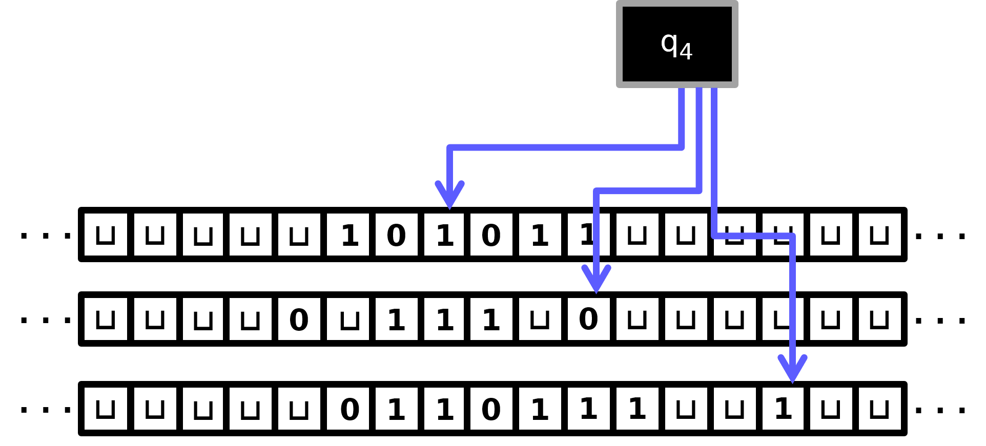
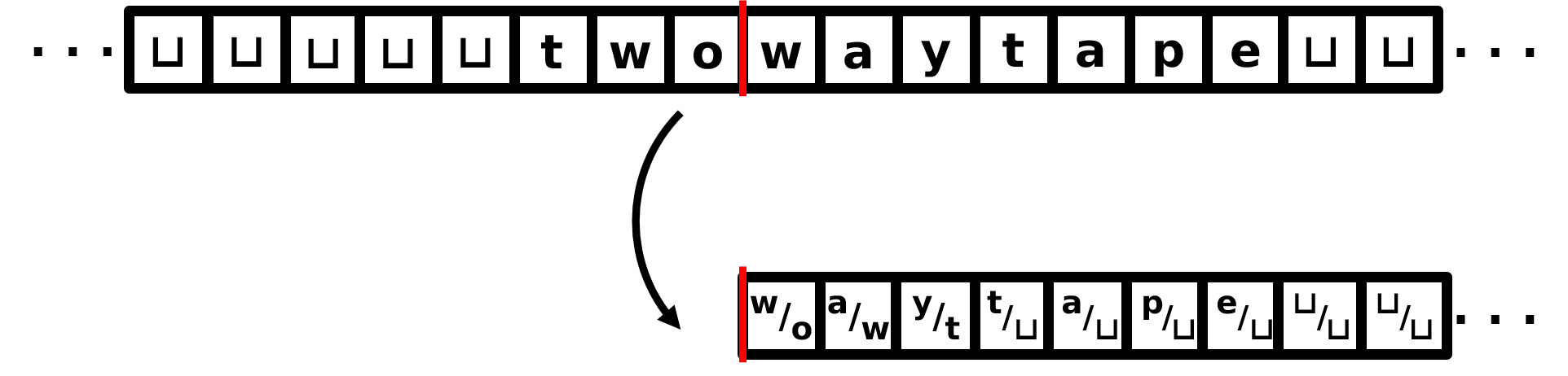
Let’s now begin to think about how we might take, say, a \(3\)-tape (call it \(M_3\)) and simulate it with a \(1\)-tape TM (call it \(M_1\)). The first idea is that we will store the contents of \(M_3\)’s three tapes consecutively on \(M_1\)’s tape, with a \(\textup{\texttt{\#}}\) punctuation mark separating them. Furthermore, we will also keep track of the three head positions of \(M_3\) on \(M_1\)’s tape using the “marking” technique from Section (TM programming tricks II: alphabet manipulation). As an example of this, suppose that at some instant in \(M_3\)’s execution, the situation is as depicted in Figure. Then at the analogous instant in \(M_1\)’s simulation, its single tape will have the following contents: \[\textup{\texttt{\#}}\mathtt{101}^{{}^{\!\!\bullet}}\mathtt{011} \textup{\texttt{\#}}\mathtt{0}\sqcup\mathtt{111}\sqcup\mathtt{0}^{{}^{\!\!\bullet}}\textup{\texttt{\#}}\mathtt{0110111}\sqcup\sqcup\mathtt{1}^{{}^{\!\!\bullet}}\textup{\texttt{\#}}\] We will call this the “compression” of \(M_3\)’s tapes; it’s similar to writing down the configuration of \(M_3\) (as you hopefully defined it in Exercise (\(k\)-tape TM semantics)), except that the state of \(M_3\) does not appear anywhere on the tape. Instead, in the simulation, \(M_1\) will keep track of \(M_3\)’s state using its own state. Note also that \(M_1\)’s head position will not directly correspond to any head position from \(M_3\). The tape head of \(M_1\) will roam freely around the tape in the effort to simulate \(M_3\).
Assuming the running time of \(M_3\) is \(T(n)\), it means that on inputs of length \(n\), \(M_3\) only has enough time to write at most \(T(n)\) symbols on each of its \(3\) tapes. In turn, this means the compressed \(M_1\) tape always has at most \(3T(n) +4 = O(T(n))\) symbols on it.
We now describe the simulation of \(M_3\) by \(M_1\).
Initialization Component.
The first stage of \(M_1\)’s operation will be to convert its initial tape (which, by definition, just has the input \(x\) written on it) into the “compressed” version of what \(M_3\)’s initial tape would be. That is, if for example \(x = \mathtt{input}\), then the first thing \(M_1\) must do is convert its tape contents to \[\textup{\texttt{\#}}\mathtt{i}^{{}^{\!\!\bullet}}\mathtt{nput}\textup{\texttt{\#}}\sqcup^{{}^{\!\!\bullet}}\textup{\texttt{\#}}\sqcup^{{}^{\!\!\bullet}}\textup{\texttt{\#}}\] It is not too hard to design a bunch of dedicated states at the “beginning” of \(M_1\)’s code to accomplish this (i.e., to write in the extra \(\textup{\texttt{\#}}\)’s and marked symbols). If the input length is \(n\), then this stage of \(M_1\)’s code will take \(O(n)\) steps (mostly for walking to the end of the input to write the \(\textup{\texttt{\#}}\sqcup^{{}^{\!\!\bullet}}\textup{\texttt{\#}}\sqcup^{{}^{\!\!\bullet}}\textup{\texttt{\#}}\) at the end). Let’s assume this first stage finishes by walking back to the left end of the tape; this takes another \(O(n)\) steps.
Head scan Component.
Now the simulation can begin. A major component of simulating one step of \(M_3\) is having \(M_1\) figure out the \(3\) symbols under \(M_3\)’s tape heads. Once \(M_1\) figures this out, since it will also be “remembering” \(M_3\)’s current state using its own state, \(M_1\) will know all it needs to know to update its compressed tape contents according to one step of the simulation. For this part of the simulation, roughly speaking the TM will have the head scan rightward, noticing and “remembering” the marked cell (using state), until it comes to the first \(\textup{\texttt{\#}}\). At this point, e.g., \(M_1\) would be in a state called something like \[q\textit{-M3-in-state-q4-and-head1-reading-}\mathtt{1}\textit{-and-scanning-right-for-head2}.\] In this state, \(M_1\) keeps scanning rightward, noticing and “remembering” the marked cell in the second segment of the of the compressed tape. For example, if it has found the marked cell but not yet the second \(\textup{\texttt{\#}}\) symbol, it might be in a state called \[q\textit{-M3-in-state-q4-and-head1-reading-}\mathtt{1}\textit{-and-head2-reading-}\mathtt{0}\textit{-and-scanning-right-for-hashtag}.\] Again, having found the second \(\textup{\texttt{\#}}\) symbol, \(M_1\) will continue to the right until it comes to the third marked symbol. Once it finds it, \(M_3\) can move on to the next component of the simulation. At this point, it will have just transitioned into a state called something like \[q\textit{-M3-in-state-q4-and-head1-reading-}\mathtt{1}\textit{-and-head2-reading-}\mathtt{0}\textit{-and-head3-reading}{\mathtt{1}}.\] Note that there is a rather enormous proliferation of states in \(M_1\); among others, we need a couple of states for every quadruple of \(M_3\)-state-and-\(3\)-tape-symbols! Also observe that the time for this “Head scan Component” is bounded by the length of \(M_1\)’s tape contents, which by Note (Compressed tape bound) is \(O(T(n))\).
Simulate one step Component.
Having worked out what is under all \(3\) tape heads, and “knowing” what state \(M_3\) is in, \(M_1\) can now update its compressed tape. This component is somewhat similar to the Head scan Component. \(M_1\) first brings the tape head to the left end of the tape. Then it scans rightward until it hits the first marked symbol. At that point it can: (i) change the symbol underneath the mark, as dictated by what \(M_3\) would write on its first tape; (ii) move the mark one cell to the left, or to the right, or not at all, depending on whether \(M_3\)’s first tape head would move L, R, or S. There is a catch here — what happens if \(M_3\) wants to move the tape head outside the boundaries of the two \(\textup{\texttt{\#}}\) symbols? We will mention how to deal with this catch below. For now, let’s not worry about it and go on. Having handled \(M_3\)’s first tape, \(M_1\) can scan rightward again till it comes to the next \(\textup{\texttt{\#}}\), and then repeat for the second tape: find the marked symbol, replace it, and adjust the mark. The same goes for the third tape. Finally, \(M_1\) can change the state of \(M_3\) that it is “remembering”, again according to how \(M_3\) would change state. It would then head leftward to find the first \(\textup{\texttt{\#}}\), starting out in a state called something like \[q\textit{-M3-now-in-state-q7-and-scanning-leftward-for-third-hashtag}.\] The overall time to execute this single step of the simulation is again proportional to the length of \(M_1\)’s tape, which by Note (Compressed tape bound) is \(O(T(n))\).
The Catch — overrunning the delimiters.
Let’s return to the issue of what happens if \(M_3\) wants to move a tape head onto a blank outside the boundaries of its current tape contents. In this case, \(M_1\) would not have sufficient “room” on its compressed tape. The solution is simply to open up a cell of space. For example, suppose \(M_3\) is trying to move its \(2\)nd tape head to the right, and this would spill the marker onto the \(3\)rd \(\textup{\texttt{\#}}\) marker on \(M_1\)’s tape. In this case, \(M_1\) enters into a subroutine that copies remainder of the tape one cell to the right (similar to the subroutine in the “stretching” algorithm, Proposition (“Stretching” the input)), opening up a new cell on its tape, into which it places a \(\sqcup^{{}^{\!\!\bullet}}\). Note that \(M_1\) will have to use “state” to remember for which tape it’s opening up a new tape cell, and whether it’s opening it up on the left or the right. As for running time, note that shifting the tape contents doesn’t take time more than twice the length of the tape, which we know is \(O(T(n))\). Thus even if \(M_1\) has to handle this “catch” all \(3\) times, the total amount of time it adds to one step of the simulation is at most \(O(T(n))\). So the time for a single simulation step is still \(O(T(n))\).
Summary.
In the way described above, \(M_1\) simulates \(M_3\) step by step. On inputs of length \(n\), we saw that each step of \(M_3\) takes \(O(T(n))\) time for \(M_1\) to perform, and \(M_3\) has \(O(T(n))\) total steps. Since the Initialization Component took time \(O(n)\), this means the total running time of the simulation is \(O(T(n)^2) + O(n)\). This is just \(O(T(n)^2)\) (unless \(T(n) \ll \sqrt{n}\), but we can ignore this case for the reasons described in Note (Sublinear time)). This completes our sketch of the proof of the following theorem:
For any \(k\), a \(k\)-tape Turing Machine \(M\) with running time \(T(n)\) can be simulated by a usual \(1\)-tape TM \(M'\) with running time \(O(T(n)^2)\). (The constant hidden in the \(O(\cdot)\) depends on \(k\).)
It is significantly more convenient to program multi-tape TMs than it is to program single-tape TMs. Happily, Theorem (Simulating multi-tape TMs by 1-tape TMs.) tells us that anything we can solve efficiently with a multi-tape TM we can also solve “almost” as efficiently with our official model of \(1\)-tape TMs. (Well, if you count quadratic slowdown as “almost”.) Let us give an example illustrating this.
There is a \(2\)-tape TM deciding the \(\textbf{Palindromes}\) problem with running time \(O(n)\).
(Sketch.) Recall that on input, say, \(\mathtt{amanaplan}\), a \(2\)-tape TM starts out like this:
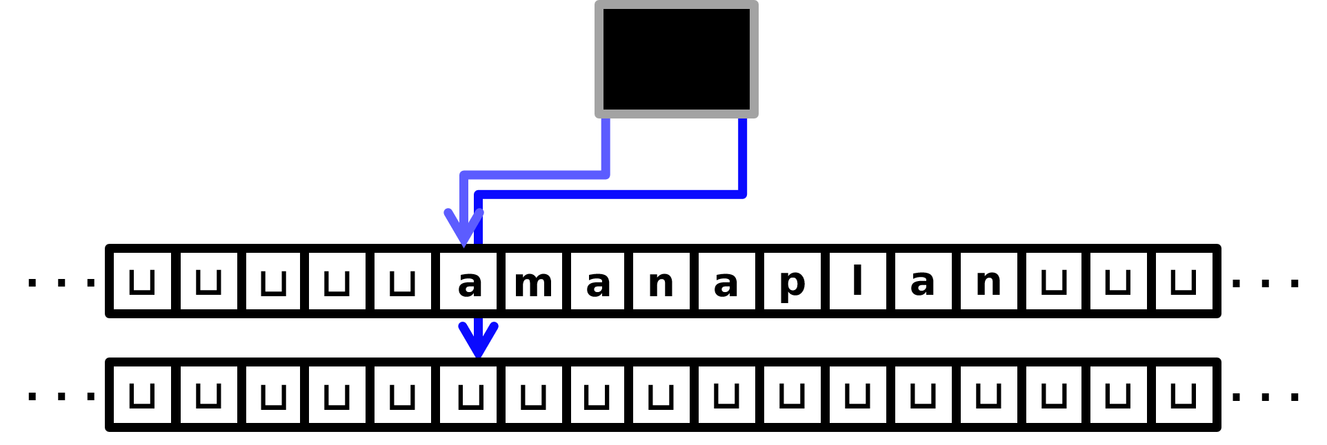
The idea of the TM is:
Walk the \(1\)st tape head to the end of the input, while keeping the \(2\)nd tape head in place. This is \(O(n)\) time.
Walk the \(1\)st tape head back to the beginning of the tape, while at the same time copying the symbols being read onto the \(2\)nd tape. This is also \(O(n)\) time, and now the TM’s tape contents would look like this:
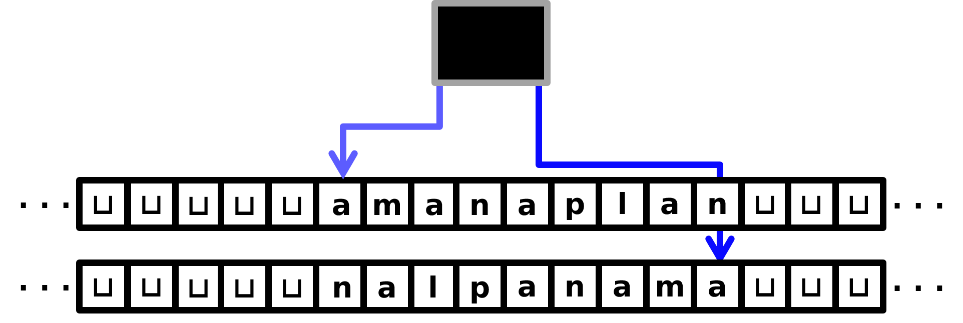
Walk the \(1\)st tape head to the right, and the \(2\)nd tape head to the left, comparing symbols as they go. If ever two symbols are distinct, reject; otherwise, if the tape heads reach blanks at the same time and all symbols matched, accept. This is also \(O(n)\) time.
This \(O(n)\) running time for solving \(\textbf{Palindromes}\) seems more “realistic”, at least in comparison with the kinds of algorithms/running-times we’re used to in algorithms courses. Recall in Example (Morphett simulator) we considered a \(1\)-tape TM solving the \(\textbf{Palindromes}\) problem, and it took \(O(n^2)\) time. In fact, this is optimal for \(1\)-tape TMs, as Frederick C. Hennie showed in 1965. (The proof is not too hard; it would take half a lecture, or a bit less.)
(Hennie, 1965.) Any \(1\)-tape TM solving \(\textbf{Palindromes}\) requires at least \(\Omega(n^2)\) running time.
Since \(\textbf{Palindromes}\) is solvable on a \(2\)-tape TM in \(O(n)\) time, Hennie’s result shows that the quadratic slowdown that Theorem (Simulating multi-tape TMs by 1-tape TMs.) gives for converting \(2\)-tape TMs to \(1\)-tape TMs can’t be improved upon.